This function is best for when you have multiple limitations (criteria) you need considered when adding values.

Are you feeling like you have a good handle on how SUMIF works? Do you understand the difference between Range and Sum_range? Great, because now we’re going to move things around a bit but maintain the definitions we’ve established thus far.

For this example, we want to know how many bonuses were paid out to employees not in Management and exclude the CEO and VP.

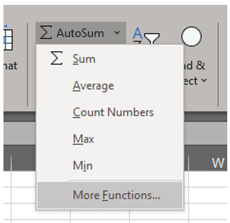
As with before, go to either the Home ribbon in the Editing group or to the Formulas ribbon in the Function Library group, click the dropdown by the sigma symbol (Σ) for AutoSum, and choose More Functions from the dropdown.

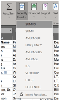
Note: If you’ve recently used this function, navigate to the Formulas ribbon in the Function Library group. rather than clicking the dropdown by the sigma symbol (Σ) for AutoSum, You’ll see a star icon titled Recently Used. Use the dropdown here to select the desired function.

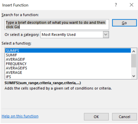
The Insert Function dialog box will appear. If you have used the function recently, it will appear on the list where you can click it and then click OK. Otherwise, type in the box where indicated the function you want to use.

This will prompt the Function Arguments dialog box, which is specific to the type of function you have chosen. This is reflected in the upper left corner of the box.

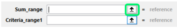
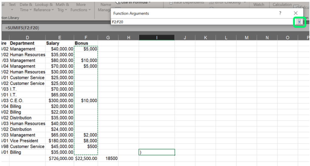
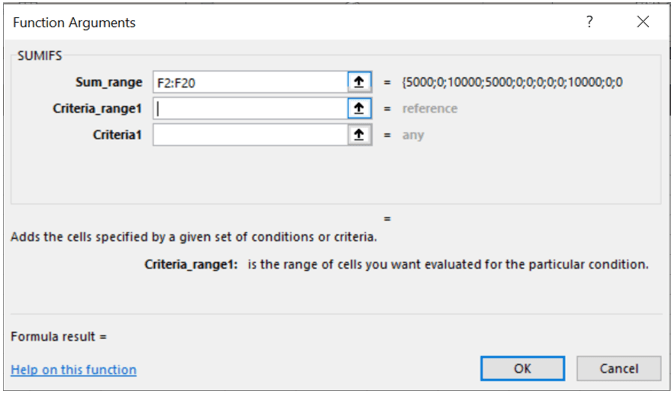
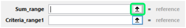
You’ll note Sum_range is now a required field along with Criteria_range1. Remember that all mandatory minimum requirements are bolded. For this function to work, you must have at least these lines complete. The Sum_range is the area of cells that will be added together. Click the up arrow to the right of the Sum_range box.

This will return you to the spreadsheet with a minimized popup. Select the Sum_range and click the down arrow when complete.

You will return to the full Function Arguments dialog box. Your Criteria must be listed on the spreadsheet so that the system can view a range for that Criteria. This area will be the Criteria_range1. This limitation does not change whether you are working with text or values. In fact, SUMIFS works best with text in mind.

Note: Since SUMIFs works well with text, I recommend using dropdown lists [NR1] for entries with repeated text, which the system is set to search for in IF-type formulas. if the formula is set to search for “management” and someone has typed in “mgmt,” “manager,” or some other variant or misspelling, the system will give false results. The dropdowns exist to standardize input[NR2] .

Notice that the moment you click in Criteria_range1, a third line appears: Criteria1.

Click the up arrow next to Criteria_range1.

You will again return to the spreadsheet with the minimized popup. Select the Criteria_range1, the area where the information for the Criteria will be found, and click the down arrow when complete.

Because we’re working with text for the limitation, we have two options: we can type in the word Management or click one of the instances where it appears on the spreadsheet. A few things to be careful of here: first, typos. If a single instance is misspelled, it won’t be counted. Second, if this is a living document where an individual’s title could change or a person leaves the company, then it would be a bad idea to use any one individual as a reference cell. The safest move for this formula is to type in the word Management. You do not need to type in quotation marks when using the wizard. Excel will automatically add them.

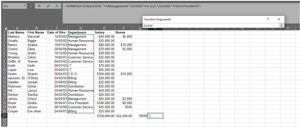
In this formula we’re telling the system to exclude the word Management which mean anything that does not match or equal  (≠), remember this is an equation, the word Management should be included. However, the does not equal symbol  (≠), according to Excel, doesn’t exist. As a replacement, when something should be excluded, the does not equal symbol is represented by <> prior to the text or number as in the image below.

You may have noticed the formula result at this point. If we clicked OK now, we would still be including the VP and CEO.

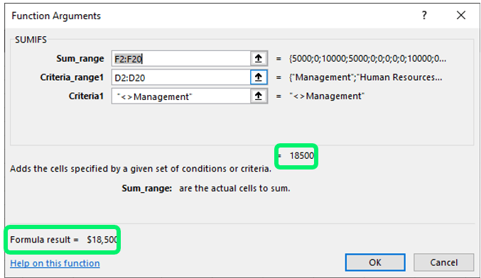
At this point, we’ve created an alternative to the example we used in SUMIF to determine the total of bonuses paid to managers but with the following formula. Notice we used the equals sign this time.

=SUMIFS(F2:F20,D2:D20, “=Management”)

If you recall, however, we decided we want to see all bonuses paid to those not in any kind of management role, which would include the CEO and VP. This is where further criteria and ranges come into play. When you clicked on Criteria1, an optional Criteria_range2 appeared. That range is on our spreadsheet, so we’ll use the up arrow again.

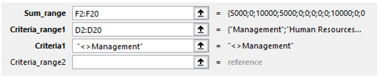
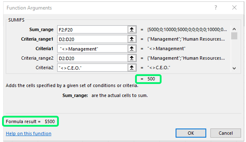
For this example, Criteria_range2 and Criteria_range2 will both be the same as Criteria_range1. You could either copy the first range and paste in the next two or follow the procedure for indicating the range as before. The Criteria can be typed in for Criteria2 as indicated in the image below.

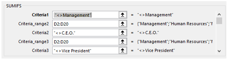
If you use the scroll bar on the right of this dialog box, you’ll see that you can keep adding criteria.

We only need the first three for the resulting formula.

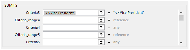
=SUMIFS(F2:F20,D2:D20, “<>Management”,D2:D20,”<>C.E.O.”,D2:D20,”<>Vice President”)

The formula is now complete. There is now a result ($500) previewed in the dialog box. Click OK.

Below are the various examples for this function.

Function	Formula	Example
SUMIFS single criteria	=SUMIF(sum_range, criteria_range1, criteria1)	=SUMIFS(F2:F20,D2:D20, “=Management”)
SUMIFS multiple criteria	=SUMIF(sum_range, criteria_range1, criteria1, [criteria_range2, criteria2], [criteria_range3, criteria3],…)	=SUMIFS(F2:F20,D2:D20, “<>Management”,D2:D20,”<>C.E.O.”,D2:D20,”<>Vice President”)