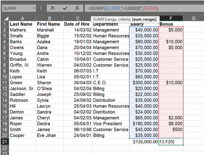
Use this formula when you want to add numbers in a range but only if they meet or do not meet certain criteria. That criteria can be text or values. Today we’ll focus on values. Let’s say we have the following table.

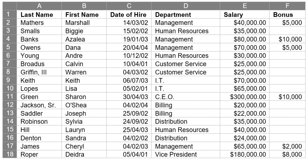
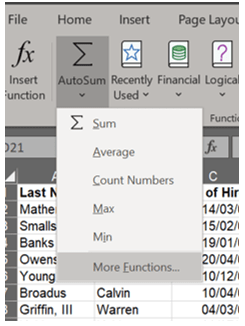
In this table, we want to determine the total of all salaries paid under $100,000. Rather than using SUM and removing lines 11 and 18, we can use SUMIF. This equation allows for a range and criteria. To use it, click the cell where you want the total to appear, then either type =SUMIF or, on the Home ribbon in the Editing group, click the dropdown by the sigma symbol (Σ) for AutoSum and choose More functions.

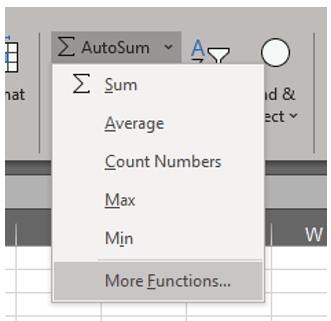
You can also go to the Formulas ribbon in the Function Library group, click the dropdown under the sigma symbol (Σ) for AutoSum, and choose More functions from the dropdown.

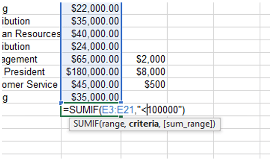
I will cover each of these methods, but first let’s look at manually typing the formula. When you type the formula in a cell, a popup wizard will remind you of the basic requirements for the formula. As mentioned, the minimum requirements needed for SUMIF are the range and criteria. We’ll be adding only the values in column E: =SUMIF(E2:E20). Next, to specify that we only want amounts under $100,000, we’ll type a comma followed by “<100000” – remember to include the quotation marks in the formula and to enter a closed parenthesis at the end. The formula won’t work without the quotation marks. The final formula will look like this: =SUMIF(E2:E20,”<100000″).

The staff salaries under $100,000 total $726,000.

Some of you might be looking at this screenshot and wondering about that [sum_range]. Why did I skip it in the initial tutorial? It’s optional at this point. For our original goal (totaling salaries under $100,000), we only needed one range and one criterion. Let’s head back to our table and I’ll explain further.

Column F shows the bonuses paid out over and above the base salary as listed in Column E. Say we want to determine the total amount of all bonuses paid to employees earning less than $100K. Rather than using SUM and figuring out individually which lines apply, as in the image below, we can use SUMIF with two ranges and one criterion.

We’ll use that same formula, =SUMIF(E2:E20,”<100000″), but this time we’ll use the formal wizard by either going to the Home ribbon in the Editing group or to the Formulas ribbon in the Function Library group, clicking the dropdown by the sigma symbol (Σ) for AutoSum, and choosing More Functions from the dropdown.

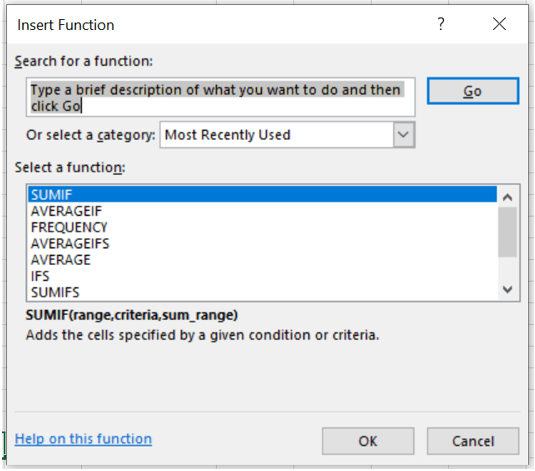
The Insert Function dialog box will appear. If you have used the function recently, it will appear on the list where you can click it and then click OK. Otherwise, type in the box where indicated the function you want to use.

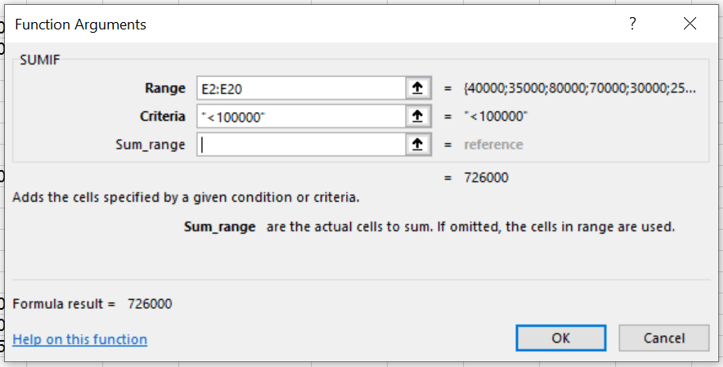
This will prompt the Function Arguments dialog box that is specific to the type of function you have chosen. This is reflected in the upper left corner of this dialog box.

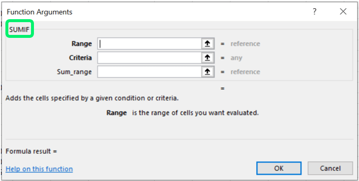
As you can see here, this box includes areas for the Range, Criteria, and optional Sum_range. The mandatory minimum requirements of Range and Criteria are bolded. This is the only visual indication that you must have at least these lines complete for the function to work.

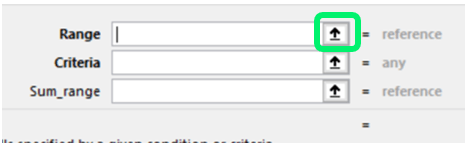
The Range is where we are pulling the information that will be judged: in this case, column E, which lists the salaries. Rather than typing the information in the box, click the up arrow next to it.

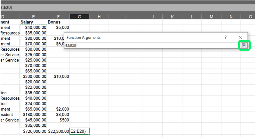
You will now return to your spreadsheet with a minimized popup. Select the Range and click the down arrow when complete.

This will return you to the full Function Arguments dialog box. If your Criteria is listed on the spreadsheet, you may click the up arrow for Criteria and select the cell(s) that list(s) the limitation. In this instance, the limitation or judgment is that we only want to look at salaries less than $100,000. This can be typed in the Criteria line as <100000.

Note: Do not type the comma in a number like this: <100,000. It confuses Excel, which thinks we’re adding either further criteria or a Sum_Range in the wrong place.

Notice that you did not need to type quotation marks when using the wizard. Excel will automatically add them.

What we’ve entered so far is telling the system to add only salaries that are under $100,000. The result is previewed in this box twice.

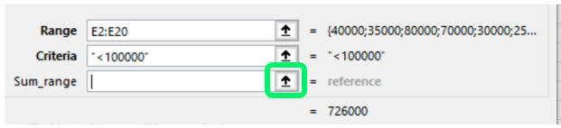
Remember, however, that we decided we want to see all bonuses paid to those earning less than $100,000. This is where the second range ([Sum_range]) comes into play. These are the numbers that will be added together. That range is on our spreadsheet, so we’ll click the up arrow again next to the box associated with Sum_range.

Now select the Sum_range.

This should be the same size (number of rows) and shape (number of columns) as the Range. If the two are different, you may run into problems. For instance, if the Range is one column but the Sum_range is three columns, the actual Sum_range that the system will look at will be reduced to one column to match the size of the Range. this means that if we kept column E but were reviewing multiple years of bonus payouts and selected columns F, G, and H (pretending those had bonus payout info), Excel would only add the information in column F.

Click the down arrow when complete.

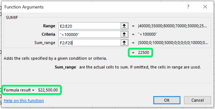
The formula is now complete. As before, the result is previewed twice in the dialog box. Click OK.

If you click on the cell the with the final formula, it will read:

=SUMIF(E2:E20,”<100000″,F2:F20)

To reiterate, the formula tells the computer to add the numbers in column F to the total of all bonuses paid to individuals earning less than $100,000 in column E for a grand total of $22,500. (This is 7.5% of the CEO’s annual salary, and I explain how I calculate that here.)

Below are the various examples for this function. I will cover how to use this formula with text on Friday.

Function	Formula	Example
SUMIF with numbers	=SUMIF(range, criteria)	=SUMIF(E2:E20,”<100000″)
SUMIF with text	=SUMIF(range, criteria, [sum_range])	=SUMIF(E2:E20,”<100000″,F2:F20) =SUMIF(D2:D20,”Management”,F2:F20) =SUMIF(D2:D20,”<>Management”,F2:F20)