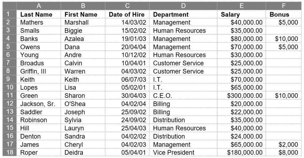
We’ve covered how to do sumifs with number limitations. But what if we wanted to see the total of all bonuses paid only to managers, using the data in our spreadsheet?

Start by going either to the Home ribbon in the Editing group or to the Formulas ribbon in the Function Library group, clicking the dropdown by the sigma symbol (Σ) for AutoSum, and choosing More Functions from the dropdown.

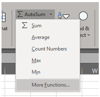
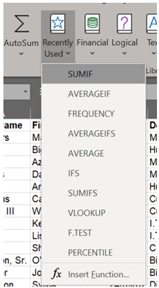
Note: If you’ve recently used this function, navigate to the Formulas ribbon in the Function Library group. rather than clicking the dropdown by the sigma symbol (Σ) for AutoSum, You’ll see a star icon titled Recently Used. Use the dropdown here to select the desired function.

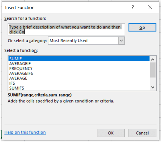
The Insert Function dialog box will appear. If you have used the function recently, it will appear on the list where you can click it and then click OK. Otherwise, type in the box where indicated the function you want to use.

This will prompt the Function Arguments dialog box, which is specific to the type of function you have chosen. This is reflected in the upper left corner of the box.

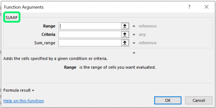
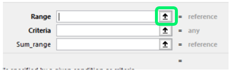
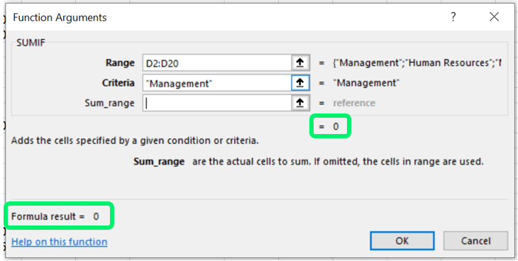
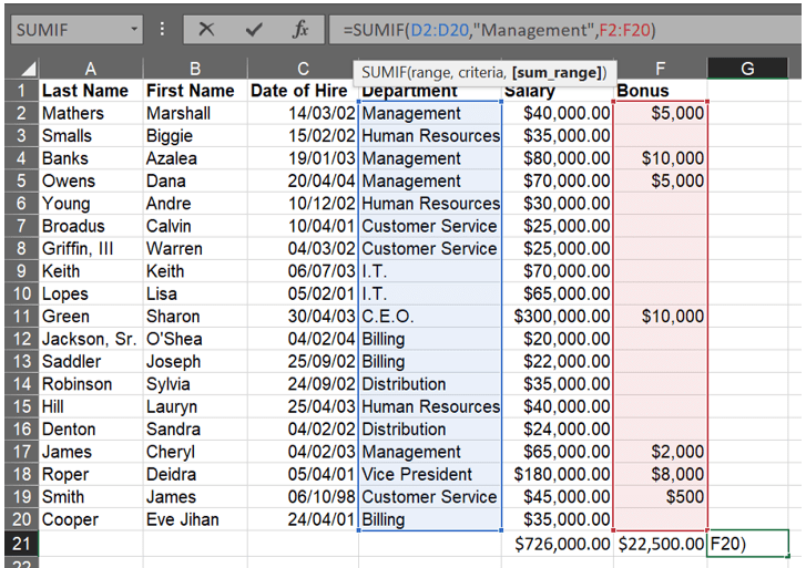
As you can see, this box includes areas for the Range, Criteria, and optional Sum_range. The mandatory minimum requirements of Range and Criteria are bolded. This is the only visual indication that you must have at least these lines complete for the function to work. The Range indicates where we are pulling the information that will be judged: in this case, column D, which lists the titles. Click the up arrow next to the line.

This will return you to the spreadsheet with a minimized popup. Select the Range and click the down arrow when complete.

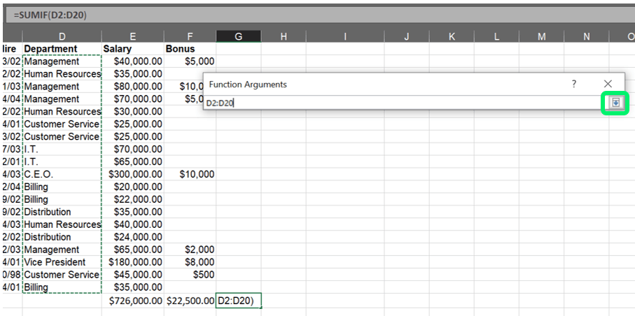
You will now return to the full Function Arguments dialog box. If your Criteria is listed on the spreadsheet, you may click the up arrow for Criteria and select the cell(s) that list(s) the limitation. Because we’re working with text for the limitation, we have two options: we can type in the word Management or click one of the instances where it appears on the spreadsheet. A few things to be careful of here: first, typos. If someone’s title is misspelled, they won’t be counted. Second, if this is a living document where an individual’s title could change or if the person leaves the company, then it would be a bad idea to use any one individual as a reference cell. Thus, the safest move for this specific spreadsheet is to type in the word Management.

Notice that you do not need to type in quotation marks when using the wizard. Excel will automatically add them.

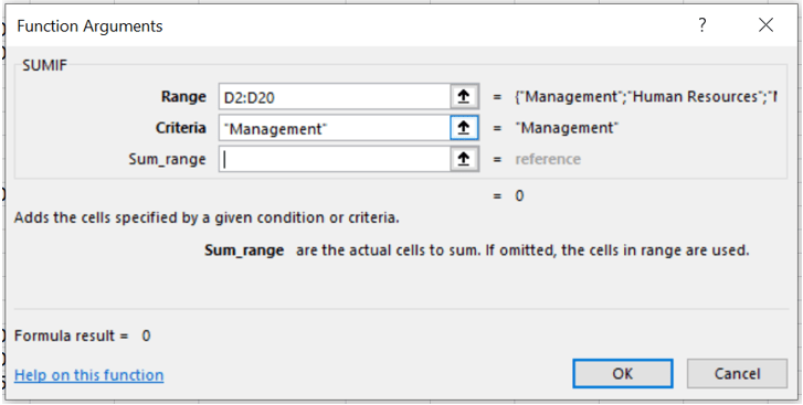
You may have noticed there is no sum result at this point, because thus far we haven’t told the system to use any numbers. If we clicked OK now, we would only receive a zero as the result—which we know is wrong.

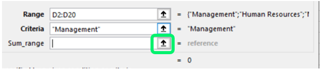
Remember, however, that we decided we want to see all bonuses paid to managers. This is where the second range ([Sum_range]) comes into play. These are the numbers that will be added together. This range is on our spreadsheet, so we’ll use the up arrow next to Sum_range again.

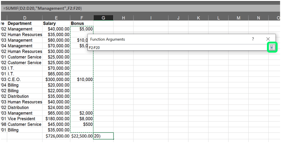
Next, select the Sum_range.

This should be the same size (number of rows) and shape (number of columns) as the Range. If the two are different, you may run into problems. For instance, if the Range is one column but the Sum_range is three columns, the actual Sum_range that the system will look at will be reduced to one column to match the size of the Range. this means that if we kept column D but were reviewing multiple years of bonus payouts and selected columns F, G, and H (pretending these had bonus payout info), Excel would only add the information in column F.

Click the down arrow when complete.

The formula is now complete. There is now a result, which is previewed in the dialog box. Click OK.

If you click on the cell with the final formula, it will read:

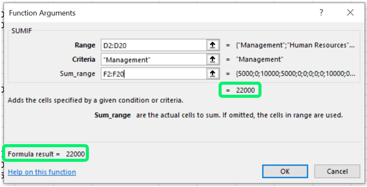
=SUMIF(D2:D20,”Management”,F2:F20)

To reiterate, the formula tells the computer to determine who is a manager based on the Criteria of Management, as listed in the Range of Column D, and to add the bonuses as listed in column F of only those individuals, the total of which is $22,000.

What if we want to exclude managers? Simply add <> to the formula:

=SUMIF(D2:D20,”<>Management”,F2:F20)

This generates a result of $18,500. The eagle-eyed will notice that this formula would include the CEO and VP. For sums with multiple criteria, you’ll need to use SUMIFS which I’ll cover on Monday.

Below are the various examples for this function.

Function	Formula	Example
SUMIF with numbers	=SUMIF(range, criteria)	=SUMIF(E2:E20,”<100000″)
SUMIF with text	=SUMIF(range, criteria, [sum_range])	=SUMIF(E2:E20,”<100000″,F2:F20) =SUMIF(D2:D20,”Management”,F2:F20) =SUMIF(D2:D20,”<>Management”,F2:F20)